This post is part of series – Posts 1 and 2

Summary:

• Starting with data exploration of the dataset
• We will likely need to do some data cleaning:
  • Most of the columns are numeric, but nearly all have at least one null value
  • There are possible duplications / overrepresentation of certain weeks
  • 2 columns may have 0 as a default rather than an actual reading in some cases
• Co-correlation of features may make modeling challenging depending on the algorithm

So I was unable to devote the amount of time I needed to be able to learn compute vision, but this competition is far simpler so I think it will allow us to build some tooling to simplify and automate tasks.

The goal of this competition is to develop a supervised model predicting to CO2 emissions in Rwanda. Since the data is tabular and primarily numerical it will make interpretation and communication simpler.

As much as I would like to dive straight into modeling we will do the responsible thing and start with some data exploration. Specifically, we will perform data quality checks, review distributions, and look at univariate correlations with our target. All of the code will be in this git repo if you want to view it.

The first thing I did was create a .py file to make this process repeatable as it is something we will want to do with most datasets. Since we are doing data exploration I thought it would be fun to name it data_de_gama.py :). There are a handful of methods in the class and those allow us to find that there are 75 columns in our feature set and only 1 of them is non-numeric. Of the 74 numeric columns, 70 have at least one null / NaN value.

It also worth scanning through the histograms of the data. I won’t bore you with all of them, but a couple I found interesting are:

The histogram of records by week number show double the number on the first, middle, and last week of the year:

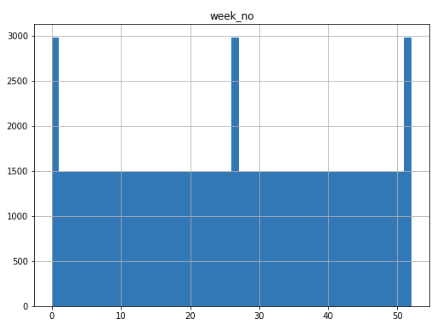
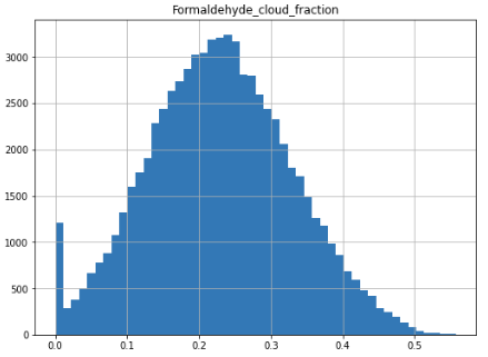
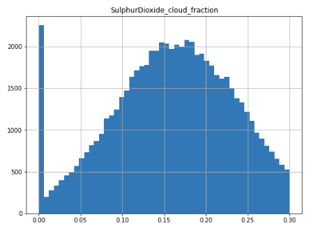
This could indicate duplicate records or at least overrepresentation of data at specific times of year, but it turns out I screwed up and coded the number of bins to 50 so a couple of weeks “tied” and made it look like there was double counting. There are also two distributions which have a spike of values at 0 which makes me question whether those are accurate readings or if 0 is a default value on at least some of them:

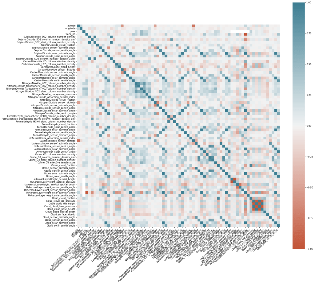
Finally I used some code from Drazen Zaric’s article on correlation matrices using Seaborn to generate the matrix below. I have only scanned it, but much of the high correlation I see are with intuitively related features, e.g. SO2 density and SO2 density 15 kilometers away. I need to add the target variable back into the dataset to look for correlations, but that will come later. For now, it is enough to know there will be some co-correlations we may need to address.