Kaggle Playground s3e20 – Post 1

This post is part of series – Posts 0 and 2

My goal with this series of posts is to step through the development of a model in this friendly competition as well as the development of tooling to make future model development faster and more repeatable. To that end, I have tried to start from a beginner’s mindset to hopefully make this more instructive.

The goal of this exercise is to predict the carbon dioxide (CO2) emissions in Rwanda for 2022 based on information gathered at nearly 500 sites across the country from 2019 – 2021. It seems likely that CO2 emissions would follow a long-term trend and seasonality throughout the year which typically means a time series is a good option for generating accurate predictions. The dataset also has other indicators of carbon emissions and so we could use a model to understand the relationship between CO2 and those features to make predictions; most likely through some form of regression as the target is numeric and continuous. The good news is that computers do not get tired so we can do both a bunch of different ways to see what makes the best predictions and iterate our way to, hopefully, more accurate predictions.

So where we left off last time was that we had some potential data issues we needed to work through, but a dataset that was mostly numeric with the sole exception of an identifier column at the beginning of the dataset. In that case, full steam ahead, let’s make some predictions.

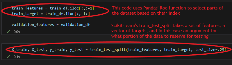
To measure the quality of our predictions data scientists typically split their data into two sets, one to develop their models on and the other to test the output / predictions of that model. The intuitive reason is that a model will perform best when making predictions about data it has already “seen”, but the way one uses models in reality is nearly always to make predictions about data that is new to the model. We will be using scikit-learn’s train_test_split method to do this randomly, to remove bias, and efficiently, to save us from writing a little code.

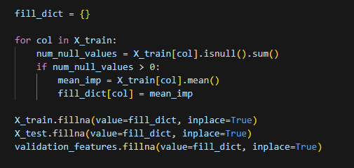
Using the data_de_gama package we put together in the previous post we can see that 70 of our 74 columns have at least 1 null value and of our roughly 60K rows one set of features has nearly 100% null values, the UV aerosol layer height group, and many of the others have null values of 10K+ records. It seems like data imputation is going to be our biggest challenge.

The simplest data imputation method is probably to just use the mean of the column so let’s do that and then create a baseline model using a simple linear regression. SKLearn has a built-in method for imputing using means, but where is the fun in that? Let’s iterate through the dataset ourselves and update missing values to the mean of the values we do have. It is important that we are using only information from the train set so you will see that we are updating the test set using the mean from the train set. Conceptually, this matches what would happen when we are making a prediction on a new record; we would only have information on past data we have seen to impute.

Using the default linear regression from SKLearn and measuring performance using our test set we get an r-squared 0.04, not good. But wait a minute; we moved too quickly. One of our features, week_no, is ordinal but the number of the week does not really express a magnitude difference; is the last week of the year 52x larger than the first? The same argument can be made about year as well, but for now I am going to keep that numeric as we know we need to create predictions for years outside of our build sample and having that be categorical will make that difficult.

To make week_no categorical we will use one-hot encoding. Data encoding will have to be a deeper topic on another day, but one-hot encoding transforms a single feature into n columns where n = the number of unique values for the features. Then, each column is set to 0 except for the one that corresponds to the value for that record. For example, when we one-hot encode our week_no column it will get split into 52 columns representing each week and for a record with week_no = 40 each column will be set to 0, except for the column corresponding to week 40, something like week_no_40, which will be set to 1.

When rerunning the flow and creating a linear regression of the one-hot encoded dataset the r-squared on the test set 0.03 which is essentially the same as the model on our unencoded dataset, especially since I created new train and test sets.

Let’s try one more thing to gather some information about our dataset; we will use a different algorithm to try and capture non-linear relationships in the data. Let’s fit a random forest regressor from sklearn and see where that gets us.

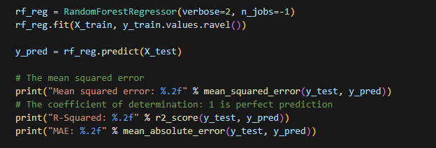
After running the code above we get an r-squared 0.95 which is very good and seems to indicate there is complexity in the relationships in our data that are not captured by the linear regression. In subsequent posts we will explore using a time series to make predictions, combining / ensembling predictions, and tuning hyperparameters if time permits.